
Finally had a chance to play around with Kaggle challenge, and bike sharing demand seems to be the easiest to tackle - no domain expertise required or atleast very minimal.
This is going to be Part 1 where I'll go over how I apply minimal statistical knowledge to extract features. Well, extraction and selection to be exact. From these features, I fed them into Random Forest (from Scikit-Learn) which hopefully will be covered in Part 2. The result I got so far is mediocre, I plan to play around with features and try different algos later when I have the time. My final target is to get score below 0.5 or around 0.4 at best before I give up :( If some of the reasoning are wrong let me know, although I have background in Actuarial Science, it has been quite a while.
Feature selection
I will be using R to toy around with the data.
Since this is going to be a regression problem (predicting a continous value), I would like to start simple with linear regression to see how things first.
> str(bike)
'data.frame':	10886 obs. of  14 variables:
 $ datetime  : Factor w/ 10886 levels "2011-01-01 00:00:00",..: 1 2 3 4 5 6 7 8 9 10 ...
 $ season    : int  1 1 1 1 1 1 1 1 1 1 ...
 $ holiday   : int  0 0 0 0 0 0 0 0 0 0 ...
 $ workingday: int  0 0 0 0 0 0 0 0 0 0 ...
 $ weather   : int  1 1 1 1 1 2 1 1 1 1 ...
 $ temp      : num  9.84 9.02 9.02 9.84 9.84 ...
 $ atemp     : num  14.4 13.6 13.6 14.4 14.4 ...
 $ humidity  : int  81 80 80 75 75 75 80 86 75 76 ...
 $ windspeed : num  0 0 0 0 0 ...
 $ casual    : int  3 8 5 3 0 0 2 1 1 8 ...
 $ registered: int  13 32 27 10 1 1 0 2 7 6 ...
 $ count     : int  16 40 32 13 1 1 2 3 8 14 ...
 $ time      : Factor w/ 24 levels "00","01","02",..: 1 2 3 4 5 6 7 8 9 10 ...
 $ day       : Factor w/ 7 levels "Friday","Monday",..: 3 3 3 3 3 3 3 3 3 3 ...
time and day are some of the variable that I extracted from datetime. I could do so for month as well. There is no statistical basis behind this, it's just purely from intuition/knowledge. But, we will let stats decide if these features are worthy.
> model1 <- lm(count ~ season + holiday + workingday + weather + temp + atemp + humidity + windspeed, data=bike)
> summary(model1)

Call:
lm(formula = count ~ season + holiday + workingday + weather +
    temp + atemp + humidity + windspeed, data = bike)

Residuals:
    Min      1Q  Median      3Q     Max
-335.81 -102.67  -31.95   66.44  677.02

Coefficients:
             Estimate Std. Error t value Pr(>|t|)
(Intercept) 135.79052    8.71016  15.590  < 2e-16 ***
season       22.75882    1.42662  15.953  < 2e-16 ***
holiday      -9.15872    9.27009  -0.988 0.323181
workingday   -1.14953    3.31527  -0.347 0.728795
weather       5.93872    2.61924   2.267 0.023389 *
temp          1.84737    1.14210   1.618 0.105796
atemp         5.63120    1.05057   5.360 8.49e-08 ***
humidity     -3.05684    0.09262 -33.003  < 2e-16 ***
windspeed     0.77762    0.19999   3.888 0.000102 ***
---
Signif. codes:  0 ‘***’ 0.001 ‘**’ 0.01 ‘*’ 0.05 ‘.’ 0.1 ‘ ’ 1

Residual standard error: 155.8 on 10877 degrees of freedom
Multiple R-squared:  0.2609,	Adjusted R-squared:  0.2604
F-statistic:   480 on 8 and 10877 DF,  p-value: < 2.2e-16
Our R-squared is not that great. Maybe we can improve this by excluding some features. Usually features with * is considered as important when evaluating the model. One thing to note is that atemp (feels like) has 3 *'s while temp does not have any. This is quite misleading. temp should also be equally important. However, because the correlation between temp and atemp is 0.9849481 (highly correlated), the other information is already being 'captured' by the other variable. So deleting one of this feature will result in minimal loss of information.
Let's take a look at humidity. The co-efficient is negative - the relationship between count and humidity is inverse, the higher the humidity the lesser the bike rental. Since I am not a weather expert, I'm not sure how true is this, but let's see it on a graph so we can confirm this.
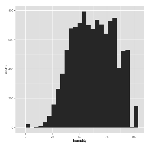
Well, the bike rental does get lesser as humidity increases although not smoothly (maybe there are some other factors influencing bike rental at this humidity level).
Another thing that I would like to do is to actually breakdown the rental between the registered and casual and to see if timings are actually affecting them. Registered user might use bike for works, and casual might use for leisure purpose. Let's see this on graph.
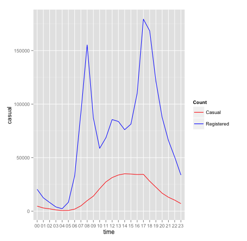
Looking at the graph, we can confirm our assumption. We can actually do a separate model to predict for casual and registered. Some of the features might remain the same, but for time, we might model them differently. Once we have the count for casual and registered, we can total them to get the predicted count.
These are some of my thought process when given data. I applied the same simple methodology for any other features like windspeed, day (Sunday is somehow important), etc. Try to analyze the data and later feed them into a model.